Sat 7-7-18 Big Pic: AII: The American Association of Individual Investors
A Quantitative Method for Asset Allocation
by Joseph Harding
Article Highlights
· Conventional rebalancing readjusts the portfolio back to the
predetermined target allocation for stocks.
· The quantitative method considers not only the target allocation
but also the prevailing valuation of stocks and the relative valuation of
bonds.
· Returns are enhanced for portfolios holding allocations of 50%,
60% and 70% to stocks; volatility is reduced for equity allocations up to 90%.
An
individual investor must decide how to allocate portions of their portfolio
among different asset classes, such as stocks, bonds or cash. A diversified
portfolio allocated among different asset classes has been proven to be an
excellent strategy for obtaining good returns over the long term, with the
added benefit of reduced volatility (i.e., avoiding large changes in portfolio
value) over the short term.
|
TAKE A PEEK
at all the member benefits AAII has to AAII is a nonprofit association dedicated to investment education. |
Indeed, AAII conducts an ongoing Asset Allocation Survey , with results
updated every month (www.aaii.com/assetallocationsurvey).
The survey measures the percentage holdings of members in five asset
categories: stock funds, stocks, bond funds, bonds and cash.
Conventional
Method for Asset Allocation
So how
does an investor go about determining the appropriate asset allocation for
their portfolio? There are two generally accepted guidelines for making this
determination.
The first guideline is that an investor must determine their
tolerance for risk. In other words, how willing are you to endure large swings
in portfolio value over the short term in exchange for potentially higher returns
over the long term? If you determine that you are willing to endure large
swings in portfolio value over the short term, then a higher percentage of
stocks compared to bonds or cash in your portfolio would be appropriate. If, on
the other hand, you determine that you are not as willing to endure large
swings in portfolio value over the short term, then a lower percentage of
stocks compared to bonds or cash in your portfolio would be appropriate.
The
second guideline is based on the expected retirement date of the investor. An
investor who is many years away from retirement should have a higher allocation
to stocks compared to bonds or cash. However, an investor who is either retired
or is only a few years away from retirement should have a lower allocation to
stocks compared to bonds or cash. Indeed, this is the idea behind the various
target date funds that are available today.
After
determining the appropriate asset allocation for your portfolio, it is not wise
to simply “set it and forget it.” Over time, the value of one asset class will
likely change compared to other asset classes. This means that over time, the
asset allocation of your portfolio will also change compared to your original
target allocation. Therefore, it is recommended that an investor should rebalance
their portfolio at least annually. During the rebalancing process, portions of
portfolio assets that have increased in relative value are sold, with the
proceeds invested in assets that have decreased in relative value. The result
is that the portfolio is readjusted back to the original target allocation
after the rebalancing is completed.
The
Quantitative Method
The
conventional method for asset allocation described so far has been proven over
time to be a good model for individual investors to follow. But what if there
is a better way?
When an
investor rebalances their portfolio, what if the investor adjusts their actual
target allocation after rebalancing based on not only their target allocation
but also the current prevailing relative value of the stock and bond market?
In the
quantitative method described herein, the allocation to stocks would be equal
to the investor’s target allocation if the current prevailing valuation of the
stock market is historically average compared to the current prevailing 10-year
Treasury note yield. However, the allocation to stocks would be greater than
the investor’s target allocation if the current prevailing valuation of the
stock market is historically below average compared to the current prevailing
10-year Treasury note yield. The allocation to stocks would be less than the
investor’s target allocation if the prevailing current valuation of the stock
market is historically above average compared to the current prevailing 10-year
Treasury note yield.
Stock Market
Valuation
A well-known method for determining the valuation of the U.S.
stock market (specifically the S&P 500 index) is the cyclically adjusted
price-earnings ratio, or CAPE ratio. This ratio, invented by Robert Shiller of
Yale University, compares the current level of the S&P 500 to its average
earnings over the last 10 years, adjusted for inflation. A high CAPE value
indicates that the stock market is overvalued, while a low CAPE ratio indicates
that the stock market is undervalued. A spreadsheet that includes all of the
relevant data for calculating CAPE is publicly available at www.econ.yale.edu/~shiller/data.htm.
The quantitative method for asset allocation described here is
based on the data contained in this spreadsheet but does not use the calculated
CAPE Shiller from the spreadsheet directly. Instead, the quantitative method
uses a 20-year period of earnings for calculating CAPE (denoted as CAPE20) and
also takes into account the current S&P 500
dividend yield compared to the current 10-year Treasury note yield.
Taking
the S&P 500 dividend yield and the 10-year Treasury note yield into account
makes logical sense. Low bond yields compared to their historical average (as
has been the case for the last several years) should support a stock market
with a higher than average CAPE. The opposite should be true if bond yields are
high compared to their historical average.
Quantitative
Method Formula
The
following formula is used in the quantitative method for determining the actual
allocation to stocks during rebalancing:
Stock
allocation = [target stock allocation + (2 × CAPE avg) – (2 × CAPE20)] × K
Where:
· Stock allocation is the actual stock allocation used by the
investor during rebalancing, in percent;
· Target stock allocation is the investor’s target allocation
to stocks;
· CAPE avg is the average value of CAPE20 over the last 600
months (50 years);
· CAPE20 is the cyclically adjusted price-earnings ratio over
the last 20 years; and
· K is 1.5 × (S&P 500 dividend yield ÷ 10-year Treasury
note yield).
The CAPE20 uses 20 years of earnings versus the 10 years of
earnings used in Shiller’s CAPE ratio. The S&P 500 yield can be calculated
using data from Shiller’s spreadsheet; simply divide the dividend by the
S&P 500 composite value. The 10-year Treasury yield can be found at www.multpl.com/10-year-treasury-rate/table/by-month.
|
Let AAII
Guide Your Investment Future
|
|
AAII
is a nonprofit association dedicated to investment education.
For full access to our award-winning content, classrooms, model portfolios and stock screens, please take a moment to join AAII today for only $29 — a 40% savings off our regular rate. |
Here’s
an example of how the formula works using a target allocation for stocks of
50%. As of early April 2018, the CAPE avg was 22.04, the CAPE20 was 34.29, the
S&P 500 dividend yield was an estimated 1.95% and the 10-year Treasury note
yield was 2.86%. Using whole numbers to represent the target allocation,
dividend yield and bond yield, the stock allocation formula would be:
= [50 + (2 × 22.04) – (2 × 34.29)] × (1.5 × (1.95% ÷ 2.86%)
= [50 + (44.08 – 68.58)] × (1.5 × 0.682)
= 25.5 × 1.023
= 26.09
= [50 + (44.08 – 68.58)] × (1.5 × 0.682)
= 25.5 × 1.023
= 26.09
This reflects
a 26% target allocation to stocks.
The
formula can result in values above 100% and below 0% (meaning negative values).
If the result is greater than 100%, then 100% is used. If the result is
negative, then 0% is used.
Comparison of
Results
In order
to compare the results of the conventional method to the quantitative method,
we need to first establish a model portfolio. The rules governing this model
portfolio are as follows:
1.
The portfolio
is rebalanced once per year.
2.
The stock
portion of the portfolio achieves the same return as the S&P 500, including
dividends. Dividends are not reinvested in stocks but are deposited into the
bonds/cash portion of the portfolio.
3.
The bond and
cash portion of the portfolio collectively achieves a return equal to 80% of
the 10-year Treasury note yield. This is considered to be a conservative
estimate.
Using
the above model portfolio as a basis, over the time period of 1950 through 2017
the quantitative method not only increases the average return of a portfolio
compared to the conventional method in almost every case, but the quantitative
method also reduces the volatility of the portfolio in every case studied (as
measured in the number of years with a negative portfolio return) when compared
to the conventional method.
The
benefits of increased returns to an investor are obvious. The benefits of
reduced volatility, in this case a significant reduction in the number of years
with a negative portfolio return, are more psychological. Even in years where
both models have a negative return, the losses are reduced with the
quantitative method. As an example, in 2008, an investor with a target
allocation of 70% stocks and 30% bonds/cash would have experienced a loss of
23.4% with the conventional method. That same investor would have experienced a
loss of 16.3% using the quantitative method.
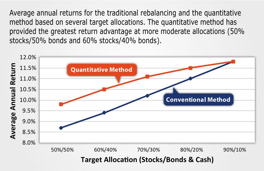
Figure
3 shows a
comparison of average annual returns between the two methods over the time
period of 1950 through 2017, depending on the investor’s target allocation to
stocks and bonds/cash.
Figure
4 shows a
comparison of the number of years with a negative return between the two
methods over the same time period, once again depending on the investor’s
target allocation to stocks and bonds/cash. Both charts are based on
calendar-year holding periods.
As can be seen in Figure
3, the quantitative method provides a distinct advantage in
returns (approximately 1% annually) for target allocations of 50%/50%, 60%/40%
and 70%/30% stocks to bonds/cash. The advantage in returns is reduced for an
80%/20% allocation. The return advantage disappears for a 90%/10% target
allocation.
Figure
4, on the other hand, shows that the quantitative method reduces
the volatility of the portfolio irrespective of the target allocation, although
the effect is reduced somewhat for higher stock target allocations.
It should be pointed out that both Figures
3 and 4 are based on an investor
rebalancing on the first trading day of October each year. This seems to be the
ideal day to rebalance compared to the first trading day of any other month. On the other
hand, the first trading day of May or June seems to be the least favorable.
However, the quantitative method still provides an advantage in returns for
lower stock allocations (i.e., 50%/50%, 60%/40% and 70%/30% stocks to
bonds/cash) no matter when rebalancing takes place. The advantage in returns
for higher stock allocations (80%/20% and 90%/10% stocks to bonds/cash) can
disappear depending on the time of rebalancing. However, the advantage of the
quantitative method in reducing the volatility of the portfolio is not
significantly affected by the rebalancing date for any target allocation.
Let’s
look at another scenario. What if an investor were able to achieve higher
returns on the bonds/cash portion of their portfolio (e.g., by holding
higher-yielding bonds), for example 120% of the 10-year Treasury note yield? As
expected, the average annual returns are increased for both the conventional
and quantitative methods, but the annual returns are increased by a wider
margin for the quantitative method. The difference in annual returns between
the two methods increases from 0.3% to 0.6%, depending on the investor’s target
allocation. In this scenario, the quantitative method continues to provide significantly
reduced volatility compared to the conventional method.
The Test of
Time
Figure
3 shows
average annual returns for the quantitative method compared to the
conventional method over a time period of 68 years (1950 to 2017). Is it
possible that the quantitative method was only better than the conventional
method for a brief period of time during that period? For example, did it
outperform in the 1950s but hasn’t offered a significant advantage since then?
My
analysis shows that irrespective of the target allocation to stocks, the
quantitative method provided superior returns compared to the conventional
method in the 1950s, 1960s, 1970s, 2000s and so far in the 2010s (i.e., 2010 to
2017).
The
quantitative method slightly underperformed the conventional method in the
1980s, and significantly underperformed in the 1990s. This result makes logical
sense.
The
1990s were famously dubbed as the era of “irrational exuberance” by Alan
Greenspan, who was chairman of the Federal Reserve Board during that period.
Dot-com stocks had extremely high valuations during this period, with a
resulting high value of CAPE20 for the S&P 500. Therefore, the quantitative
model was suggesting a lower allocation to stocks during that period. However,
stocks kept going up anyway, until they didn’t!
The next
decade of 2000 to 2009 was a dismal period for stock returns, with two major
stock market declines. In this decade, an investor with a target allocation of
90%/10% stocks to bonds/cash, using the conventional method, would have
experienced an overall portfolio loss of 1% over the entire 10-year period.
That same investor would have experienced a gain of 44% if the quantitative
method was used. Although 44% is not a great portfolio return for a 10-year
period, it sure beats a loss!
|
TAKE A PEEK
at all the member benefits AAII has to offer. AAII is a nonprofit association dedicated to investment education. |
|
If an investor rebalanced at the time that these
calculations were run in early April 2018, the model would have suggested a
below-target allocation to stocks and an above-target allocation to bonds and
cash.
|
|
|
Target
Allocation
|
Suggested
Allocation
|
|
50% Stocks/50% Bonds and Cash
|
26% Stocks/74% Bonds and Cash
|
|
60% Stocks/40% Bonds and Cash
|
36% Stocks/64% Bonds and Cash
|
|
70% Stocks/30% Bonds and Cash
|
47% Stocks/53% Bonds and Cash
|
|
80% Stocks/20% Bonds and Cash
|
57% Stocks/43% Bonds and Cash
|
|
90% Stocks/10% Bonds and Cash
|
67% Stocks/33% Bonds and Cash
|
What the Model
Currently Says
As of early April 2018, the quantitative model calculates a
current CAPE20 of 34.3, with an average CAPE20 over the last 50 years of 22.0.
Therefore, the model is suggesting a below-target allocation to stocks at the
time the calculations were run. The suggested allocations can be seen in Table
1.
Looking to the
Future
Although
the quantitative method of determining asset allocation that I have described
here has been shown to provide advantages over the conventional method, it is
likely that further improvements could be made to the formula presented in this
article. Such improvements will be the aim of future research in this area.
No comments:
Post a Comment